Anormaly Detection 방법 중 하나인 Isolation Forest에 대해 알아보겠다.
IF(= Isolation Forest)는 Unsupervised Anomaly Detection 중 하나이며, Novelty 보다는 Outlier Detection 방법이다.
Anomaly Detection이 무엇인지,
Label에 따라 Supervised, Unsupervised, Semi-Supervised Learing,
Abnormal의 종류인 Novelty, Outlier 등 기본적인 것들은 이전 포스팅에 설명해놓았다.
2021.05.12 - [AI/Anomaly Detection] - Anomaly Detection by Auto Encoder
Anomaly Detection by Auto Encoder
Auto Encoder로 Anomaly Detection 하는 방법 설명 및 Kaggle 사례 소개 오토인코더로 이상치를 탐지하는 방법에 대해 설명하기에 앞서, 이상 탐지가 무엇인지 간단히 설명하겠다. 1. Anomaly Detection이란? Norma
leedakyeong.tistory.com
(IF를 이해하려면 의사결정나무(Decision Tree)를 알고있어야 한다.)
IF의 기본 컨셉은 Outlier일수록 Decision Tree에서 Root Node와 거리(Path Length)가 가깝다에서 시작한다.
예를 들어, 다음과 같은 7개의 데이터가 있다고 하자.
변수는 X 한개이다.

변수가 1개뿐이므로 1차원 그래프로 시각화하면 다음과 같다.

눈으로 봐도 g만 멀리 떨어져있는 Outlier임을 알 수 있다.
X변수로 random하게 기준을 잡아 Decision Tree를 만들면 다음과 같다.
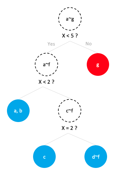
안에가 색칠되어있는 node들이 최종적으로 분리된 node들이며, 가장 말단에 있으므로 external node 또는 leaf node라고 한다.
Outlier인 g는 root로 부터 단 한 번의 질문만에 고립되었다. 반면, 다른 데이터들은 두 번, 세 번의 질문이 필요했다.
즉, 이렇게 Outlier는 Random Decision Tree의 Root node로부터 path length(=split 수)가 가깝다는 특징을 이용한 것이 Isolation Forest이다.

IF를 통해 Abnormal Score를 계산하여 Normal과 Anomaly를 구분하는데, 계산 방법은
1. Train Set으로 Random Decision Tree를 여러개 만들고(Forest)
2. Test Set에 대해 각 Data별로 모든 Tree에 대해 Root Node로 부터 Path Length를 계산한 후, 평균낸다.
3. 계산한 Path Length들로 Abnormal Score를 구하여 Outlier를 판단한다.
단,
① Decision Tree를 만 들 때 Train Set의 모든 데이터를 다 쓰지 않고 sampling해서 사용한다.
② Decision Tree를 만들 때는 Random하게 변수를 선택하고, Random 하게 Split Point를 선택하여 Split한다.
③ 모든 Data가 고립될 때까지 Split한다.
① Decision Tree를 만 들 때 Train Set의 모든 데이터를 다 쓰지 않고 sampling해서 사용한다.
Data Set이 크면 오히려 Normal Data 때문에 Tree가 Anomaly Data를 고립시키는데 방해할 수도 있다. 따라서 Sampling해서 사용한다.
또한, normal instance와 anomaly instance가 너무 가까운 경우나, anomaly instace가 꽤 많고 밀집되어 있는 경우에도 이렇게 sampling해서 진행하는 것이 효과적이다.(아래 그림 참고)

③ 모든 Data가 고립될 때까지 Split한다.
단, 실제로는 대부분의 Data가 Normal Data이므로 모든 Normal Data를 굳이 끝까지 고립시키지 않아도 잘 작동한다.
어차피 Anomaly Point만 구분하는 것이 목적이고, Anomaly Point의 Path Length는 짧을 것이기 때문이다.
(아래 Algorithm에 height limit까지만 Tree를 키우는데, 이게 그 이유.)
Random Tree를 한 개만 만들어 사용하지 않고 Forest 형태로 여러 개 만들어 평균내는 이유는 Random 때문이다.
Split 할 때 필요한 변수도, 몇을 기준으로 Split할지도 random으로 결정하기 때문에 모든 Tree의 생김새가 다를 것이다.
따라서 여러 개의 Tree를 만들어 평균내준다.
아래 이미지는 Normal Data $x_i$와 Outlier Data $x_0$의 tree개수에 따른 average path length를 나타낸 그래프이다.

1. Normal Data인 $x_i$의 path length가 당연히 Outlier data인 $x_0$보다 큰 것을 볼 수 있고
2. tree의 개수가 적을 때는 path length가 많이 흔들리고, tree 개수가 많아질수록 값이 일정하게 수렴하는 것을 볼 수 있다.
2번과 같은 이유로 하나의 tree가 아니라 여러개의 tree를 만들어 평균낸다.
모든 데이터를 고립될 때까지 Tree를 만들고, 앙상블을 통해 Forest를 만드므로 이 알고리즘의 이름이 Isolation Forest이다.
실제 알고리즘은 다음과 같다.
Training Stage(Sample Data로 Isolation Forest 생성)와 Evaluating Stage(Test Instance에 대해 Path Length 계산)로 나뉘며,
Training Stage는 다시 Decicsion Tree를 만드는 부분과 Tree들을 모아 Forest를 만드는 부분이 있다.
Training Stage

sample size는 256, tree 개수는 100개 추천. (from 논문 저자)
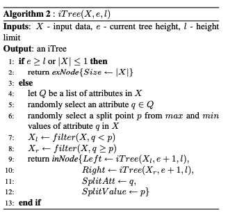
위에서 언급했듯, 원래는 모든 instance에 대해 Isolation하게 만드는 것이 원리이나, 굳이 끝까지 Isolation하게 만들 필요가 없으므로 height limit까지만 Tree를 키운 Partial Model을 만든다.
단, height limit은 $ceiling(log_2{\psi}), \psi : size \ of \ sample $ 로 세팅한다.
sample size가 n이라 할 때, tree height는 최대 n까지 커질 수 있으나, average height는 $log_2{n}$ 이다.
(Tree 만드는데 사용된 sample이 256개라면 Tree 평균 깊이는 7)
예를 들어, 다음과 같이 n=4인 sample data로 Isolation Tree를 만든다고 할 때,

아래의 왼쪽 이미지처럼 split point를 잘 못찾으면 Tree는 깊게 자라고(height $n-1$), 오른쪽 이미지처럼 split point를 아주 잘 찾으면 Tree는 얕게 자란다.height $log_2{n}$)

Evaluating Stage

Evaluating Stage는 Test Set에 대해 진행되며 Test Set의 모든 instance x에 대해 $E(h(x))$를 계산하는 과정이다.
$E(h(x))$는 instace x가 iForest 안에 모든 iTree들을 지나 계산된 $h(x)$들을 평균내면 된다.
Algorithm3에 2번을 보면 $ e + c(T.size) $가 있다.
$e$는 Root node로 부터 x instance가 속한 external node까지의 edge 개수이고(몇 번 split했는지)
$c(T.size)$는 instance가 고립되지 않았을 때 즉, height limit에 의해서 tree가 끝까지 안만들어졌거나, 값이 같아서 등의 이유로 external node에 두 개 이상의 instacance가 포함되었을 때, 실질적 depth를 계산해 주기 위해 더해주는 값이다.
고립될 때까지 tree를 만들어주어야 하는데, 효율 등의 이유로 tree를 만들다 말았으니, 끝까지 만들었다면 더 필요했을 Path Length를 계산해서 더해주는 것이다.
알고리즘에는 T가 external node면 그냥 e+c 하라고 나와있으나, 논문을 읽어보면 이러한 조건이 더 자세히 나와있다.
실제 sklearn에 구현된 코드를 보면 n<=1일 때 c=0, n=2 일 때 c=1으로 고정하고, n>=3 부터 c를 계산하여 더해준다.

$c(n)$은 external node가 n개인 BST(Binary Search Tree)에서 root부터 external node까지의 평균 depth를 구한 식이다.
즉, 만약 어떤 external node에 1개가 아닌 4개의 instance가 있다고 했을 때,
4개의 instance로 새 tree를 만든다면 external node까지 평균 path length가 $c(4)$이므로 이만큼을 더해주는 것이다.
계산 식은 다음과 같다.
$$ c(n) = 2H(n-1) - (\frac{2(n-1)}{n}) $$
$$ where H(i) = ln(i) + 0.5772 $$
$n$ : Tree를 만드는데 사용된 Sample Data 개수
$H(i)$에 0.5772 : 오일러 계수
이 계산식이 나온 과정은 아래 링크에 잘 설명되어 있다.
Unsuccessful Search
Data Structures and Algorithms with Object-Oriented Design Patterns in Java All successful searches terminate when the object of the search is found. Therefore, all successful searches terminate at an internal node. In contrast, all unsuccessful searches t
book.huihoo.com
the average depth in an unsuccessful search in a Binary Search Tree
For a research project I'm using the isolation forest algorithm. The developers of this algorithm make use of Binary Search Tree theory. They state that the average depth in an unsuccessful search...
stackoverflow.com
(참고) BST(Binary Search Tree)란?
이진탐색(Binary Search)과 연결리스트(Linked List)를 결합한 자료구조의 일종으로, 효율적인 탐색 능력을 유지하면서 빈번한 자료 입력과 삭제를 가능하게끔 고안되었다.

위 이미지와 같이 binary 형태로 가지를 뻗어나간다.
5, 8, 10, 4, 13과 같이 아래 더이상 붙어있는 node가 없는 애들을 external node(or leaf node)라 하고,
그 외의 node들은 internal node라 한다.
가장 위에 있는 11은 internal node이자 root node이다.
이렇게 계산한 Path Length로 Anomaly Score를 계산하는 식은 다음과 같다.
$$ s(x,n) = 2^{-\frac{E(h(x))}{c(n)}} $$
$x$ : instance
$h(x)$ : path length of x
$E(h(x))$ : average path length of x(모든 Tree에 대해 h(x) 계산 후 평균)
여기서 $c(n)$으로 나눠주는 것은 Sample Data 수에 따라 값에 차이가 나는 값을 Normalize해주기 위함이다.
단 3개 Data만 가지고 Tree를 만들 때와 1,000개 Data를 가지고 Tree를 만들 때 external node까지의 PathLength는 Outlier 여부를 떠나서 값 차이가 많이 날 것이며, 그 의미도 다를 것이기 때문이다.
$h(x)$는 0~n-1 값을 가지며, score는 0~1 값을 가진다.
score값이 0에 가까우면 normal, 1에 가까우면 Outlier라 판단한다.
Python에서 Isolation Forest를 적용하는 방법은 너무나도 간단하다.
sklearn에 이미 구현되어있기 때문에 그냥 가져다 쓰면 된다.

-1.1, 0.3, 0.5, 100으로 Train했고, 0.1, 0, 90에 대한 Anomaly 여부를 확인하는 코드이다.
결과는 Normal이면 1, Anormaly면 -1을 return한다.
(sklearn에서 0~1 값으로 나오는 score 계산식을 살짝 변형하여 score가 아니라 1,-1을 return한다. score_samples()로 실제 score도 뽑아볼 수 있다.)
Paper : https://cs.nju.edu.cn/zhouzh/zhouzh.files/publication/icdm08b.pdf?q=isolation-forest
sklearn IsolationForest Class github : https://github.com/scikit-learn/scikit-learn/blob/7b13a8f120a6d67112b0f50a8834d65e2258f045/sklearn/ensemble/_iforest.py
GitHub - scikit-learn/scikit-learn: scikit-learn: machine learning in Python
scikit-learn: machine learning in Python. Contribute to scikit-learn/scikit-learn development by creating an account on GitHub.
github.com
'AI > Anomaly Detection' 카테고리의 다른 글
| RaPP(Novelty Detection with Reconstruction along Projection Pathway) 구현 :: Tensorflow, mnist (7) | 2021.06.21 |
|---|---|
| Anomaly Detection by Auto Encoder (4) | 2021.05.12 |